
Chronicle 2: Meet, Follow and Understand GNSS Signals
In the previous article we explored the basics of position estimation: measuring the signal travel time and converting it into distances. And from there, with at least four satellites we solved the position and clock discrepancies.
That insight came from our road trip experiment, where we recorded data and saw how different phones sometimes disagreed on the provided route.
But that raise a deeper question. Before any of that math can even begin, how does the receiver get those satellite signals? By the time the signal reach the ground, they are weak, burried in background noise. The receiver has to detect the satellites, lock onto their signals in time, and stay in sync… while everything else moves.
Detecting it requires carefully designed signals and sophisticated receiver processing. So what is really happening inside the signals and the receiver?
In this chronicle we try to explain how GNSS signals are structured and how receivers use them. We will look at the components that form the signal, how it is transmitted from space, and how a receiver extracts the information needed for positioning.
To understand how receivers extract information from GNSS signals, we first need to see what these signals contain.
What is inside a satellite signal
Each GNSS satellite acts like a small radio station, continuously broadcasting a structured signal. However, the signal is not a simple radio transmission. It is well structured so that receivers can identify satellites, measure the travel time and retrieve data needed to compute the satellite position.
To achieve this, each satellite signal contains three components:
- pseudorandom noise code (PRN) which helps the receiver identify the satellite and precisely align time
- navigation message: a slow stream of data with the information needed to compute the position
- carrier wave: the underlying radio frequency that actually carries the two previous components through space
Together, these three elements form the transmitted GNSS signal, each contributing with a different piece of information that the receiver needs to completely understand the signal.
The PRN code: the satellite’s fingerprint
PRN stands for Pseudorandom Noise. Each satellite has assigned an unique identifier which is referred to as PRN.
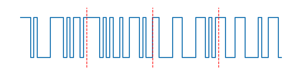
From this unique identifier, the satellite generates a spreading code which is an unique sequence of bits transmitted as part of the signal. This code is often called PRN code.
Although the sequence appears random, it is actually well defined and known in advance by GNSS receivers (this is where the “pseudo” comes from).
Each satellite transmits a different PRN code (or spreding code) for each signal it broadcast. This allows the receiver to distinguish signals coming from different satellites even though they share the same frequency band.
The spreding code also provides the key to measuring signal travel time. If you keep reading, we will decipher together how this is done.
🛰️ Think of it as each satellite broadcasting its own unique rhythm, allowing the receiver to distinguish it from all the others.
Each satellite will transmit more spreading codes (PRN codes), one for each frequency. In GPS, the PRN code code on the L1 frequency is called the C/A code. The signals from other frequency bands (e.g. L5) and other constellation such as Galileo use different types of codes, but the priciple is the same: each satellite transmits an unique code per frequency.
The navigation data: slow bits that matter
In addition to the PRN code, the signal carries a navigation message. This message is a slow data stream (50 bits per second for GPS), but carries essential information:
- Ephemerides: precise orbit parameters that tell us where the satellite was at the moment it transmitted its signal.
- Clock information: corrections for the satellite clock
- Health status: flags that inform if the satellite has any issues
This data tells the receiver where the satellite was and what time it was when the signal was transmitted.
When people talk about satellite orbits you will often hear about Keplerian elements. These are six parameters that describe an ideal Kepler orbit. In GNSS, the receiver gets those elements from the ephemeris, broadcast in the navigation message. Of course, the real orbits are not perfectly Keplerian, so the navigation message also includes small corrections to account for perturbations and clock effects. By combining the ephemeris and these corrections, the receiver can compute a precise satellite position at the moment of the signal transmission.
The carrier: the vehicle to ride from space
The third component is the carrier wave. The carrier acts as a vehicle that allows the two signals to travel at a specific frequency or radio band and reach the receiver. The ones you will see the most are:
- 1575.42 MHz (GPS L1 and Galileo E1): a common, widely supported frequency
- 1176.45 MHz (GPS L5 and Galileo E5a): a cleaner signal that is very useful when combined with L1/E1 (often called Dual-Frequency)
There are other bands, like GPS L2 and Galileo E5b/E6, but L1/E1 and L5/E5a cover what most phones use.
In navigation nomenclature, the discrete transition are called: bits in the navigation data and chips in the PRN code.
These three components are not transmitted separately. Together, they form the structured signal that is continuously broadcast by the satellite and that receivers detect and process.
How the signal is built
The components described above need to be combined and transmitted as one signal.
First, the navigation message is combined with the PRN code (or spreding code). This combined digital sequence is then modulated onto the carrier wave, allowing the signal to be transmitted from the satellite to Earth.

The transmitted satellite signal is built in two steps:
- Combine the navigation data and the PRN code
- Modulate that result onto the carrier so it can travel through space and reach the receiver
This process transforms the digital information into a physical signal that can propagate through space.
Code + Navigation message
The navigation message has a low data rate. These slow bits are mixed with the PRN code, which has a faster chip sequence. The resulting combination is our baseband message signal, s(t).
In practice, the navigation bits change slowly while the PRN code repeats continuously. This combination ensures that the signal simultaneously supports PRN measurements and data transmission.
Note: You can also find in literature that the XOR operation is a module-2 sum.

Modulation onto the carrier
Once the digital sequence is formed, it must be transmitted as a radio signal. The combined signals are at baseband. We need to put that baseband signal onto a carrier so it can propagate and fit into the allocated spectrum. This is done by modulation that will shift the signal to the frequency of the carrier.
One of the modulation used by the GNSS signals is Binary Phase Shift Keying (BPSK). In this modulation scheme, the phase of the carrier wave is shifted depending on the value of the transmitted bit. (There are fancier modulations like BOC/CBOC, but BPSK captures the core idea.)

The result is a structured radio signal that carries timing information, satellite data, and a satellite identifier. They are all embedded in the carrier wave.
Here is what that looks like mathematically (don’t worry if it seems abstract at first):
s(t) = A \cdot D(t) \cdot C(t) \cdot cos(2 \pi f_c t + \varphi)
where
- s(t): signal that the satellite broadcasts
- A: amplitude of the signal
- D(t): navigation message
- C(t): PRN or C/A code
- cos(2 \pi f_c t + \varphi): carrier; for example, f_c=1575.42 MHz for L1
Why modulation? Higher frequency carriers allow for smaller antennas and “live” in protected frequency bands reserved for GNSS signals, which avoids interference from other radio services.
We have seen how the resulting combination of the signals look like, let’s take it further and see how the receiver can actually understand them.
From space to receiver
Now that we know what the satellite transmits and how the signal is constructed, let’s follow its path from space to the receiver and see how it is processed.
After leaving the satellite, the signal begins its journey toward Earth. The satellites orbit in the Medium Earth Orbit (MEO) at an altitude of 20000 km. During the journey, it spreads out, losing its power. By the time it reaches the ground, it is delayed, attenuated and buried in noise.

🛰️ What the satellite sends
As we saw above, the signal transmitted by the satellite can be written as:
s(t) = A \cdot D(t) \cdot C(t) \cdot cos(2 \pi f_c t + \varphi)
All the information the satellite sends is packed together, creating the modulated signal your receiver hears: a precise combination of data, identity and rhythm.
📡 What the antenna receiver hears
As we said, the signal does not arrive exactly as it left the satellite. We can write the received signal as:
r(t) = A\cdot D(t - \tau) \cdot C(t- \tau) \cdot cos(2 \pi (f_c + f_D) t + \varphi) + \varepsilon(t)
Each term tells a small part of the story of how it reached the receiver:
- r(t): signal at the receiver
- A: the amplitude, weakened by distance and atmospheric attenuation
- C(t-\tau): C/A code shifted in time by \tau(code delay)
- D(t-\tau): navigation message data arriving a little late due to travel time \tau(code delay)
- cos(2 \pi \ (f_c + f_D) \ t + \varphi): carrier whose frequency f_c has been slightly shifted by the Doppler effect by f_D Hz, caused by the satellite and receiver moving relative to each other
- \varepsilon(t): all the unwanted extras; noise and errors introduced in the transmission.
Despite the signal attenuation and the changes it went through, the GNSS receivers (like our phone) are able to detect and process these signals.
To do this, the receiver performs several steps. It first tries to hear the signals and detects them. Once a signal is found, the receiver lock onto it and keeps track of it. Finally the navigation data embedded in the signal is decoded.
These steps are the core of the GNSS signal processing inside the receiver.
Inside the receiver

The receiver processes the signal in stages:
- Antenna: captures the RF (radiofrequency) signal and transforms it to an electrical signal
- Analog section of the receiver: the signal coming out of the antenna is downconverted from RF to an intermediate frequency. Then it is demodulated, i.e. we separate the carrier from the combination of the navigation message and C/A code
- Analog-digital converter (ADC): samples the signal so we can process it
- Digital section of the receiver: this is where the magic happens. The input signal (the combination of the navigation message and C/A code) goes through three steps that allow us to decode the information received from the satellite:
- acquisition: find each satellite in the noise,
- tracking: keep lock and measure precisely,
- navigation: decode the slow data to get ephemerides and clock info.
Think of it as a meet → follow → understand sequence where the receiver first finds a satellite, then follows it tightly while everything moves, and finally understands the slow data is sending.
The first of these steps, the acquisition, is the process in which the receiver discovers which satellites are visible and determines where their signals are located in time and frequency.
Acquisition: finding the satellite
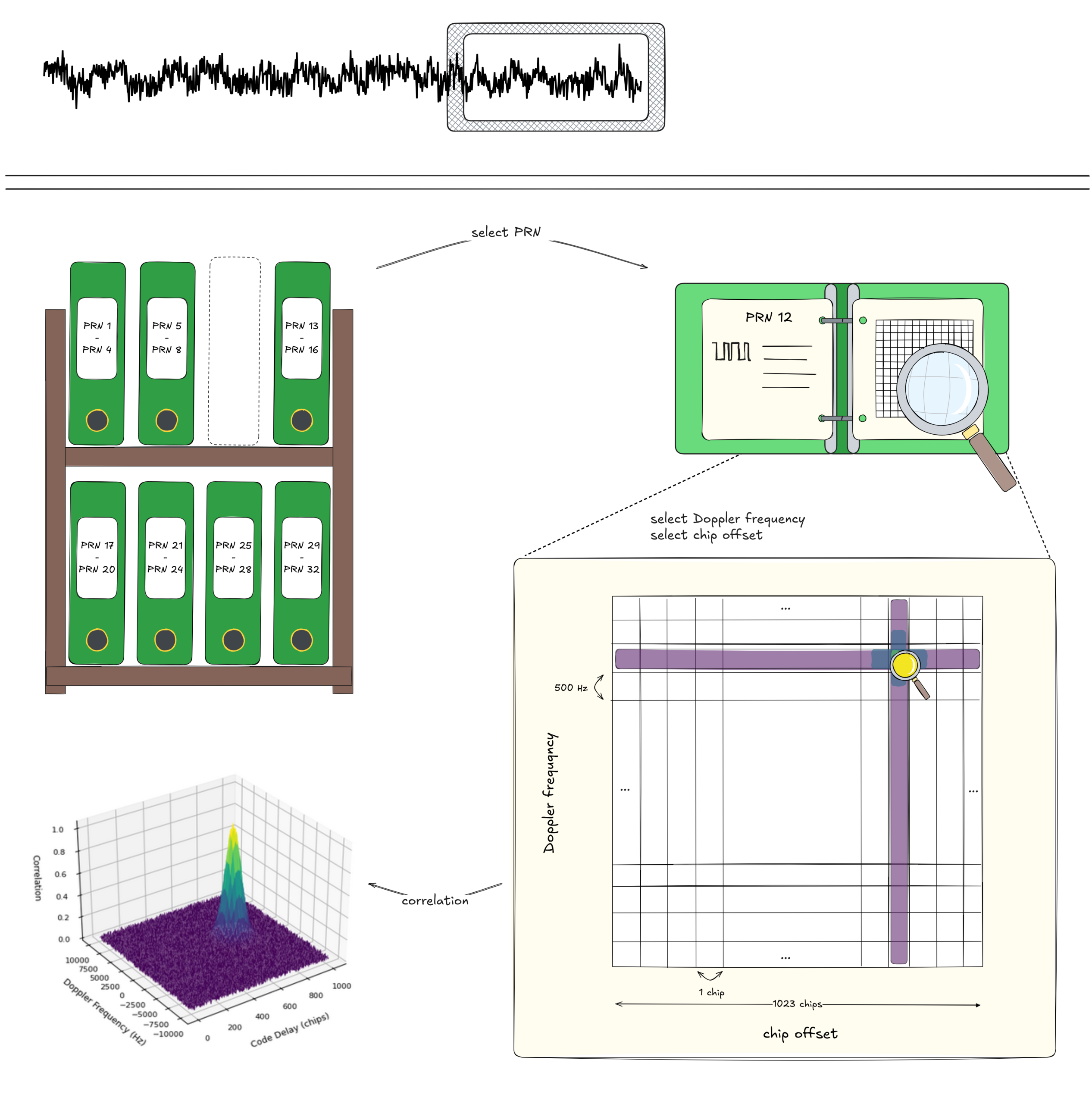
Before the receiver can measure the distance, it must first detect which satellites are present. Because the signals are weak, the receiver cannot detect them directly. It must perform a search process scanning thousands of possible code delays and Doppler frequencies.
Acquisition is the “meet” phase. Imagine trying to find one specific melody in a room full of statics. You slowly slide your tuner until the sound snaps into place.
For a successful acquisition of the signal, the receiver needs to detect which satellites are present and obtains coarse estimates of their code delay (\tau) and Doppler (f_D). For doing this, the spotlight turns to the PRN code… so it is time to shine PRN!
We remember that the key PRN characteristics are:
Unique + Pseudo Random + Noise
Because PRN codes are unique, the receiver can store a “database” of all of them from a constellation (or even multiple constellations): the incoming signal is a noisy recording and the database is a collection of known fingerprints. Then, the receiver has the task to detect which satellite fingerprints are present and roughly align them with the local copies stored in its database. But… what powers this search engine of our PRN database?
The answer is correlation.
Because PRN codes are pseudorandom, one PRN code looks like noise to any other. But if we take the correct PRN code from the database and slide it chip by chip over its chip period (1023-chip period for GPS L1, 4092 for Galileo E1), there is one alignment where the local code matches the received one. At that point, the correlation spikes… And that’s the magic, the satellite reveals itself!
Visually, this means that the correlation will have only one peak per satellite, in the grid point that matches the chip delay and doppler frequency.
Currently, the GPS constellation has 31 satellites, which in the worst case scenario means that we have 31 PRNs x 1023 chip combinations. Galileo has 32 satellites in orbit with 26 operational and for each 4092 combinations.
But there’s one more complication: the Doppler shift. This is because the satellite and the receiver are moving simultaneously, the signal shifts in frequency. Without compensating for it, the correlation peak might not be strong enough to detect. For L1 GPS, f_D is within the range of 5-10 KHz. If we search in steps of 500 Hz, we have 40 blocks, meaning 41 points to add to the searching area.
The acquisition problem therefore becomes a three-dimensional search:
PRN × code delay × Doppler frequency
Based on the values that we have seen, for GPS that means 31 PRNs x 1023 chips x 41 frequency blocks and for Galileo 26 PRNs usable x 4092 chips x 41 frequnecy blocks.
Even for a single constellation this means testing over 1 million hypotheses! Receivers speed this up with clever FFT-based methods. If you enjoy performance optimization problems you can have a lot of fun 🙂
Outcome of the acquisition phase:
For each detected satellite, the receiver knows which PRN is present and has coarse estimates of its code delay and Doppler. This is enough to move to the next phase: tracking.
Tracking: keeping lock on the signal
Once the acquisition has detected the satellite signal, the receiver knows the approximate code delay and Doppler frequency. This information allows it to move to the next stage: tracking.
Tracking is the “follow” phase. After a satellite has been found, the receiver must stay in sync with it while both the satellite and the receiver move.
The goal of tracking is to maintain a stable lock on each detected satellite and refine the initial coarse estimates of the code delay and Doppler. In particular, the receiver improves the estimate of the code delay (\tau) to sub-chip precision, and the Doppler frequency (f_D) to Hz level accuracy and begins tracking the carrier phase.
During tracking, the receiver continuously aligns the incoming signal with locally generated replicas and refines them using feedback control loops. This is where precision is gained.
To achieve this, the receiver uses feedback loops that monitor small differences between the received signal and the locally generated replica. These differences are used to adjust the local signal parameters in real time.
At this stage, the signal is characterized by these three parameters: \tau, f_D, \varphi. The receiver maintains the corresponding local replicas: \hat{\tau}, \hat{f_D}, \hat{\varphi}
The differences between the signal and replicas are:
\Delta \tau = \tau - \hat{\tau}, \Delta f_D = f_D - \hat{f_D}, \Delta \varphi = \varphi - \hat{\varphi}The role of the tracking loops is to drive these differences towards 0.
\Delta \tau \approx 0, \Delta f_D \approx 0, \Delta \varphi \approx 0Different loops handle different aspects of the signal. The Delay Lock Loop (DLL) refines code timing to sub-chip precision, while the Frequency and Phase Lock Loops (FLL/PLL) track Doppler and carrier phase as the relative motion evolves.
By constantly adjusting the local replicas, the receiver keeps them tightly aligned with the real signal. The output of this process is a steady stream of clean navigation bits together with precise timing and frequency observables.
Outcome of the tracking phase
The receiver achieves sub-chip code alignment, corresponding to timing precision on the order of tens of nanoseconds (roughly 30 cm in range), and maintains continuous lock on the satellite signal.
Navigation message: “where and when” is the satellite
Once the receiver has established stable tracking, it can begin decoding the navigation message embedded in the signal. This is the moment when the receiver moves from detection to understanding.
During acquisition and tracking, the receiver estimates a delay between the received signal and its local replica. This delay is continuously refined during tracking.
However, this delay is only a relative time, it tells the receiver how much the signal is delayed, but not when it was transmitted. To turn this into a physical distance, this delay needs to be place into an absolute timeline. This is exactly what the navigation message provides: a link between the signal and absolute system time.
What does the navigation message provide?
The navigation message gives also the last pieces needed to turn the timing information into position
- time when the signal was transmitted
- position of the satellite at that moment
Transmission time: the “when”
The navigation message is structured as a nested timing hierarchy, where each layer builds on the previous one: message, frame, subframe, bits, PRN code, chips.
We take the example of GPS L1 PRN code, called C/A code. For GPS L1 C/A, the structure looks like this:
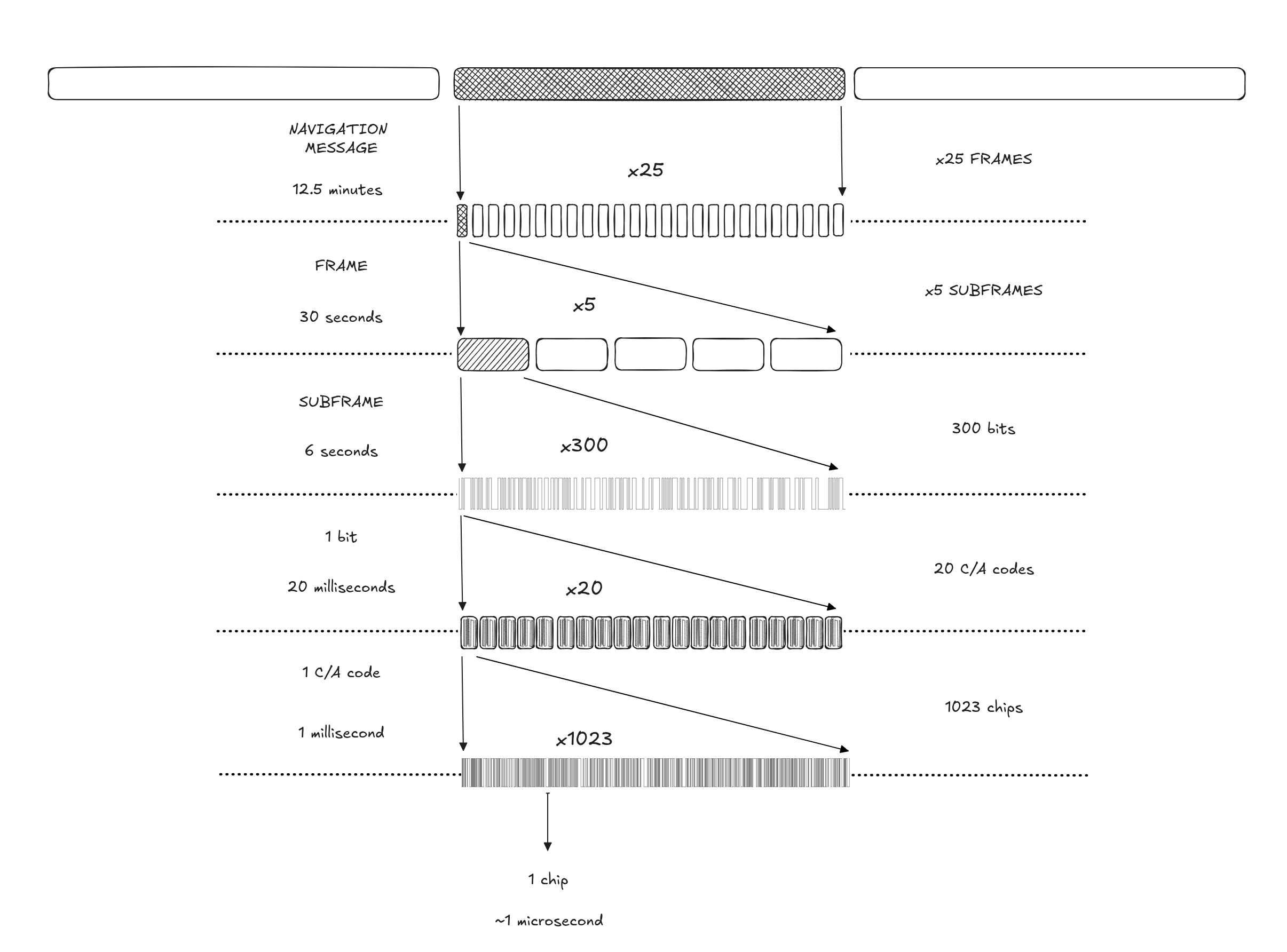
| Level | Duration | What it contains |
|---|---|---|
| Navigation message | 12.5 minutes | 25 frames |
| Frame | 30 seconds | 5 subframes |
| Subframe | 6 seconds | 300 bits of navigation data |
| 1 bit of subframe | 20 milliseconds (ms) | 20 C/A code periods |
| CA code (PRN code) | 1 milliseconds (ms) | 1023 chips |
| CA chip (PRN code bit) | ~1 microsecond (us) | Smallest PRN unit |
For other constellations the lengths are different, but the principle is the same. For Galileo for example, the navigation message length is 10 minutes for F/NAV and 12 minutes for I/NAV.
Each bit, code period, and chip in the navigation message provides a finer level of timing resolution. In case of GPS L1 C/A code:
- A bit of navigation data lasts 20 ms (6 s / 300 bits)
- Each bit contains 20 C/A code periods (1 ms each)
- Each C/A code consists of 1023 chips (~1 microsecond resolution)
This hierarchy allows the receiver to refine time from seconds down to microseconds.
Outcome of the navigation message phase
Thanks to the acquisition and tracking phase, the receiver is able to align to the navigation data. With it, we can go up in the nested hierarchy to get the exact time when the message left the satellite. However, we first need to decode the slow bits of the navigation data, where that information and much more are waiting for us.
Time offset at nanosecond resolution
Acquisition keeps us locked onto the signal to the microsecond level, and with the tracking phase, we go even further, reaching the nanosecond level. However, we still have to understand how to translate such accurate resolution into a timestamp.
Intuitively, we might expect to start with a coarse estimation, placing that timestamp on a general time scale like UTC. However, because the receiver needs to make sense of the satellite signal from the ground up, we actually do it the other way around. We estimate the fine grained offset first, and add it to the coarse reference later.
Once we know the satellite, the chip offset, and the Doppler frequency, we can estimate the precise code delay, tau (note that this tau will include the additional nanoseconds estimated during the tracking phase). Then, we can move one level up, counting the number of complete PRN codes until we reach a bit transition in the navigation message. Let’s call this count of PRN codes M.
Once we are aligned with the bits, we can start making sense of the data. To find the true beginning of the message (the subframe), we scan for a specific, recognizable sequence of bits that acts like a handshake. Counting the bits from that starting point gives us N bits.
By putting M, N, and \tau together, and knowing the exact time units associated with each one, we can calculate our highly precise time offset 💪
Establishing the coarse time
Aligning with the navigation data gives us a very accurate perception of where we are within the signal, but the receiver still needs to place that microsecond level moment onto a precise timeline to figure out exactly when the message left the satellite.
To do this, the navigation message includes a built-in time reference. But here is the catch: each GNSS operates on its own internal time scale!
- GPS Time (GPST) started on January 6, 1980
- Galileo System Time (GST) started on midnight August 22, 1999, UTC
These times are expressed as:
- Week number: number of weeks since the start time
- Time-of-week (TOW): a continuously increasing timestamp within the current week
Each subframe in the navigation message includes a TOW value, which provides a coarse transmission time reference.
Reconstructing the satellite time
The receiver can now combine the coarse time with the nanosecond offset to finally obtain the timestamp when the signal was generated by the satellite:
t_s = t_{b} + (N-1) \cdot 20 \cdot 10^{-3} + (M-1) \cdot 10^{-3} + \tau
where
- t_s time at the satellite when the signal was transmitted.
This is our satellite timestamp 🥳 - t_b broadcasting transmission time.
This is the result of combining the week number (multiplied by seconds in a week) plus the TOW. This is ffirst time the receiver gets an absolute time. - N identifies the navigation bit within the subframe: 6 s / 300 bits → 1 bit lasts 20 ms
- M identifies the C/A code within that bit: 20 CA codes in 1 subframe bit → 1 C/A code duration 1 ms
- \tau time delay representing the number of chips in the CA code
By combining the transmitted time of the subframe, the bit and code indices, and the code delay, the receiver now has an absolute time and the exact moment when the signal was transmitted.
It was a long ride, but we finally know where t_s comes from! And going through all of this also gave us some additional knowledge. This will help us with those infamous “known variables” of the system of equations that allow our phone to know where it is.
Let’s move on to understand where the satellite is: x_i, y_i, z_i.
Satellite positions: the “where”
Now that we have cracked the code on when the signal was sent, it is time to figure out exactly where the satellite was floating in space when it sent it.
If we decode the navigation message, we will see that it contains a multitude of information needed not only to compute the satellite’s position but also for other essential tasks:
- Ephemeris parameters: orbital information of the transmitting satellite
- Clock parameters: time references and clock corrections
- Health status: indicators showing if the satellite is operating properly
- Additional corrections: data such as ionospheric model parameters
By plugging the ephemeris parameters into a set of standard orbital equations, we can compute the exact position of the satellite in its orbit.
And there we have it, those most wanted x_i, y_i, and z_i coordinates! 🥳
With the satellite’s exact position known and our highly precise timestamp estimated, the receiver finally has all the ingredients needed to calculate the actual distance to the satellite.
The satellites are not alone…
We know the satellite broadcasts its ephemeris parameters to tell us its location, but how does know where it is in the first place?
Satellites move along their orbits, experiencing slight variations that need to be monitored and corrected to properly estimate their position. They can do that because the satellites do not work alone, even if until now it seemed so.
The ground segment (counterpart to the space and user segments) is responsible for this task.
Up to this point, we saw how the receiver determines its Position, Velocity, and Time (PVT) from the satellite signals. But the satellites themselves also need accurate information about their own position and clocks.
This is achieved through a global network of ground stations that constantly receive and monitor data from the satellites. These stations estimate each satellite precise orbit and clock behavior.
In a way, this is a reverse PVT problem. Instead of the receiver determining its position from satellites, the ground segment determines the satellites’ position and clock behavior from a global network of monitoring stations.
These corrections are then uploaded back to the satellites, ensuring that the entire system remains synchronized and accurate.
What comes next?
What began as noise from orbit becomes a coherent understanding of where the satellite is, how fast is moving, and what time it is.
We know where the satellites are and when the signals were sent, but there are still some unkowns in the receiver time and the synchronisation.
So, how do we align them and how we compute psuedoranges? What errors affect this measurement?
Stay tuned for the next article!
🧪 Curiosity Challenge: Acquire a GNSS signal
It is now time to see how a GNSS receiver actually hears the satellites.
In this curiosity challenge, you are the GNSS receiver! Detect the satellite by correctly choosing the PRN, and acquire its signal by finding the correct combination of code delay and Doppler frequency.
Try the interactive game below and see if you can lock onto the satellite 🕹️
(Tip: you are looking for the highest correlation)
📚 Recommended Reading

Position, Navigation, and Timing Technologies in the 21st Century: Integrated Satellite Navigation, Sensor Systems, and Civil Applications, Volume 1.
We recommend Chapter 15 for the explanations on signal tracking.
Buy on Amazon
⚙️ GNSS in your Phone
Do you know which GNSS hardware is in your phone?
Check some of the HW bellow:
- GNSS Chips usually from Qualcomm, Broadcom
- Tiny antennas such as those from Ezurio, Molex
- Clock TCXO, typical ones are Kyocera or TXC 7M Series
- DSP units are usually embedded in the main processor, e.g. Hexagon (Qualcomm)
Check real examples on iFixit teardown
⚙️ Tools
- XOR tool – create your own XOR cipher
- Understand BPSK – this simulator has a clear explanation