
GNSS Series — Part 1 of 3 · All parts · Next: Chronicle 2: what would it be?
Chronicle 1: How Does Your Phone Know Where It Is?
Ever wonder how your phone magically knows where you are whether you’re hiking, driving, or walking in your city? In this first Chronicle of our GNSS series, we take you on a real road trip and unpack the science behind smartphone location: GNSS satellites, trilateration, clock bias, and more.
This GNSS journey starts with a real journey, one of our Christmas trips when we drove from the Netherlands to Italy. While planning the route our engineering curiosity kicked in: How does our phone know where we are? Android and iPhone don’t always agree.
Yes, we’re a perfect Android-iPhone team…if by perfect you mean we each think the other made the wrong choice. 🙂 That was enough to get our engineering brains buzzing. Could we turn a 12-hour drive into a GNSS experiment? …Of course we could.
So let’s start with the big question: how does our phone know where we are?
GPS, GNSS & MEO
The answer lies in something you might already know, GPS. But GPS is just one member of a much bigger family called GNSS, or Global Navigation Satellite System. GNSS includes several systems developed by different countries, the main ones being GPS (USA), Galileo (Europe), Glonass (Russia), BeiDou (China) and Navic (India). Most GNSS satellites orbit in Medium Earth Orbit (MEO), about 20 000 km above us, circling the Earth in 12 to 14 hours.
In contrast, Low Earth Orbit (LEO) satellites move much faster, which means you need a much denser constellation to maintain coverage, since each satellite is visible for only a short time. Another type of satellites are Geostationary Earth orbit satellites, that are much farther away from Earth. These satellites circle above the Equator at a speed that matches the Earth’s rotation, so from the ground they appear to stay in the same spot.
With this in mind, we started looking into what we could do for our trip and see whether we could set up a GNSS experiment. Our available lab? Two Android phones and one iPhone. Each phone computes the position internally and uses it to “guide” us. But could we get more than just the position? Could we actually record the measurements?
Experiment preparation
Time to put our curiosity to the test. But there was a small problem: Unfortunately, iPhones restrict access to raw GNSS data. Instead, you only get the processed position (we will learn the differences soon). Android, on the other hand, gives access to all the measurements. To start logging them, all you need is an app like GNSSLogger App. You can find more details about this app and the measurements it can record on the Android developer site.
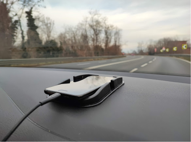
So we installed it, grabbed a phone stabilizer, basically a holder to keep the phone steady, and declared our mobile lab ready for action. For a more professional setup, we would recommend fixing it to the window or have a more solid holder, but for a first experiment, this would do just fine.
We planned the route using Google Maps as navigator and tried to stay as much as possible on the suggested route.
During our trip, we logged several tracks, pausing the recording whenever we made a stop.
If you want to upload the recorded file to e.g. Google Drive, you might need internet access. In our case, as we crossed several countries switching providers, we sometimes had issues with the connection and the file uploading.
Once we arrived at our destination, and after a well-earned rest, we finally dove into our datasets to see what we had captured.
Visualizing the results
For the analysis, we used GNSS Analysis. This app works directly with the logs from GNSSLogger and provides positioning results; it processes the raw measurements and provides the position points (and some additional parameters). You can learn more about the app and download it for Linux, Windows, or macOS from here.
Now it was time to see what data we collected. Can we use it to trace our path? We noticed some strange things along the way and we were curious to see what the data was going to reveal us.
We can keep it simple for now, without getting (yet) into details of how the position is computed. GNSS Analysis loads the file, computes the position, and outputs not only measurements but also the calculated position. A nice feature of GNSS Analysis is that it also outputs KML(Keyhole Markup Language) files, which can be easily importable into Google Earth. These .KML files contain the positions calculated by the app.
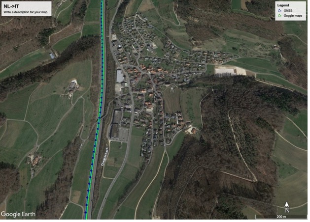
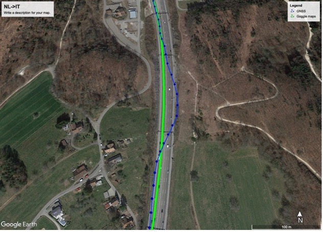
What we did was use Google Earth to look at two things: 1) the route suggested by Google Maps, and 2) the route computed by the phone, as stored in the KML file. In the screenshots below from Google Earth, the green line shows the Google Maps route, and the blue line shows the actual locations computed with the measurements from the phone. Picture 1 shows a pretty good match. But picture 2? … we definitely did not drive across that field, we stayed on the highway!
To understand what happened, we need to dig into how our position is calculated and how GNSS works.
Understanding GNSS: Trilateration, clock bias and more
As mentioned above, all the systems rely on a constellation of satellites that are orbiting in MEO. Why MEO? It is a trade-off: the higher we go, the fewer satellites we need for global coverage, but go too high and the signals get weaker.
At its core, GNSS positioning uses trilateration, similar to triangulation, but based on distances and extended into 3D.
To figure out our position, GNSS needs a coordinate frame, basically a 3D map where every point has unique coordinates. Once we have that frame, and each point has its coordinates, it all comes down to geometry. In 2D, the distance between two points in Euclidean space:
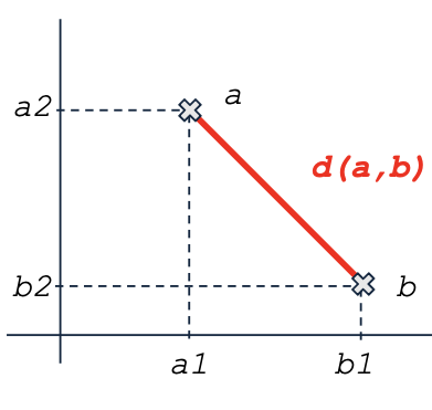
d = \sqrt{(a_1-b_1)^2 +(a_2-b_2)^2}
In GNSS, we work in 3D, so we need to add one more term:
d = \sqrt{(a_1-b_1)^2 +(a_2-b_2)^2+(a_3-b_3)^2}
Thus, the equations become:
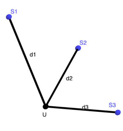
d_1 = \sqrt{(x-x_1)^2 +(y-y_1)^2+(z-z_1)^2}\\
d_2 = \sqrt{(x-x_2)^2 +(y-y_2)^2+(z-z_2)^2}\\
d_3= \sqrt{(x-x_3)^2 +(y-y_3)^2+(z-z_3)^2}\\
Simple in theory…but the challenge is getting the coordinates and time with very high accuracy.
This usually works very well if we know the distances accurately. But can we really assume this for GNSS?
GNSS Clock Bias Problem
The satellites send signals and our phone receives and decodes them (we will unpack the signals and the messages in more detail in the next Chronicles of Curiosity). In GNSS, we estimate the distance from the satellite to the user (our phone) based on the signal travel time.
distance = signal\_velocity \cdot time\_taken
- The signal velocity is the speed of light, c
- The time taken is the difference between the time the satellite transmits the signal (t_s) and the time it is received by the user’s phone (t_u).
So we get: d = c \cdot (t_u-t_s)
Sounds simple, right? Except t_s and t_u are stamped by two different devices:t_s is stamped by the satellite, while t_u is stamped by the user’s phone.
To get very accurate distances, the satellites’ clocks would need to be perfectly synchronized with our clock, which they are not. Why is that?
- The satellites have very precise atomic clocks, drifting about 1 second every hundred million years.
- The user clock (our phone) has a quartz oscillator and is far less accurate, drifting about 15 seconds in just 30 days.
This mismatch creates a clock bias unknown to the user, meaning the phone’s timestamp does not match the satellite’s. In GNSS, this is very important because even a tiny timing error changes the calculated distance: 1 microsecond error translates to a 300 m position error!🤯
Account for the difference
How do we handle the difference between the phone and satellite clocks? By adding a new variable: t_{bias} .
When the user (the phone) reads the time t_u , this value is affected by the bias. We can model it as t_u = t_r + t_{bias} .
The distance comes from the signal travel time, as we have just seen. Now, we can distinguish between two cases:
- The geometric distance (the true range):
- The measured distance (affected by the bias):
So the clock bias adds the term c \cdot t_{bias} to the measured distance. This is whyin the GNSS world, the measured distance is called pseudo-range, to explicitly emphasize that it is not the actual range and you will usually find it with the notation \rho.
How do we solve the clock bias problem? We add one more satellite. Three satellites give us position (x, y, z), and a fourth lets us estimate the clock bias between our phone and the satellites.
Let’s get accurate! When we solve the equations with three satellites, we don’t get a single point, we actually get two possible positions. Geometrically, this happens because the three spheres (the distances to each satellite) intersect in two points. One solution is near the Earth’s surface, where we expect the receiver to be. The other lies far out in space and can safely be ignored in practice.
If you want to understand better how this works, take a look at the steps below.
From Pseudoranges to Position
So we need 4 satellites, but how do we actually compute the position?
It comes down to solving a system of equations, with four satellites giving us four equations. Each one combines what we know, satellite position and pseudorange, with the unknowns, which are our position and the clock bias.
\rho_1 = \sqrt{(x-x_1)^2 +(y-y_1)^2+(z-z_1)^2} + b\\
\rho_2 = \sqrt{(x-x_2)^2 +(y-y_2)^2+(z-z_2)^2} + b\\
\rho_3 = \sqrt{(x-x_3)^2 +(y-y_3)^2+(z-z_3)^2} + b\\
\rho_4 = \sqrt{(x-x_4)^2 +(y-y_4)^2+(z-z_4)^2} + b\\
We want to estimate the user position (x,y,z) and the clock bias term b=c*t_{bias} . Each satellite gives us one equation that depends on those four unknowns. With exactly 4 satellites (and no noise), we have 4 equations and 4 unknowns -> one perfect solution. Hooray!
- But measurements are never noise free so even with only 4 satellites we do not have one perfect clean solution.
- In real life we usually have more than 4 satellites leading to an overdetermined system and the measurements are noisy. That means more equations than unknowns, which can not all be satisfied exactly. Instead, we search for the position and bias that best fit all the equations at once.
The math method that can be used to solve the system (with 4 or more satellites) is the least squares. In simple terms, what the least square does is to find the solution (point, line, curve) that minimizes the sum of squared differences between what the equations predict and what the measurements actually say.
There is one catch: the equations we have are not linear as they involve square roots. So we first turn the nonlinear system into a linear one, but only locally, around an initial guess. Meaning, we start with a very rough approximation and we slowly get close to the solution.
Position solution
The simple steps:
- Start with a rough guess for (x, y, z, b).
- Linearize the satellite equations around that guess. Tip: The linearization is done using Taylor series, but we will not go into the math here.
- Solve the resulting linear system using the least square.
- The solution of the equations gives us the correction(delta) to our position and clock bias, that we use to update our current guess. In this step, we update the guess position and the clock with the delta just computed
- Use the update guess and repeat steps 2 to 4 until the changes are very small (the solution converges)
This iterative approach is known as the Newton-Raphson method. We can think of it as a smart way to get closer and closer to the solution of a system of equations, like zeroing in on the right answer by making small, careful adjustments each time.
Inside each iteration, the linearized system of equations is solved with the least square method.
Once this is done, we get your position and your phone’s clock bias.
Is everything ready?
And just when we thought we had it all figured out… we realize that we have many “known unknowns”.
We understand how the navigator uses GNSS to estimate our position (4 satellites, linearization, Newton-Raphson), and we can rest assured about where we are. We can finally relax. But curiosity has its own way of interrupting that calm. When we look away from the moving dot on the screen and back to the equations, something feels unfinished. They work, sure, but they also raise some new questions. How do we retrieve the exact time when the signal was sent? And how do we determine the satellite positions with the accuracy we need?
🧪 Curiosity Challenge
What you need
- Android phone
- GNSS Logger app
- GNSS Analysis
- Google Earth
Steps
- Install GNSS Logger on your phone.
- Configure logging setting:
- Go to Home -> Enable all fields under Location
- GNSS log: Enable NMEA
- Rinex files: Enable Log Rinex
- Start recording
- Go to Log -> Start Log before you start
- After finishing, tap Stop&Send Log When you finish press End Log.
- The log file is stored under the default path in Android: /Android/data/com.google.android.apps.location.gps.gnsslogger/files/
- Process the data
- Open the log file in GNSS Analysis (select the .txt file)
- The software generates several figures and a .KML file in the output folder
- Visualize the route
- Open Google Earth
- Load .KML file
- Assign different colors to each track for comparison.
- Zoom into specific areas and check the accuracy differences.
📚 Recommended Reading

Global Positioning System
A great introduction covering signals & positioning. Chapter 5 details the position solution.
Buy on Amazon
⚙️ Recommended Hardware

Android phone
Buy on Amazon
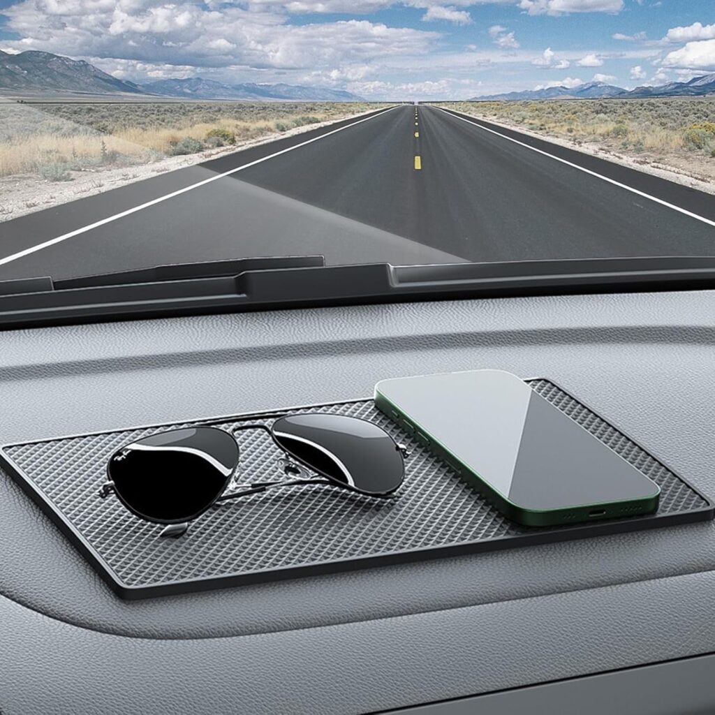
Phone holder
Keep the phone steady and in one place.
Buy on Amazon
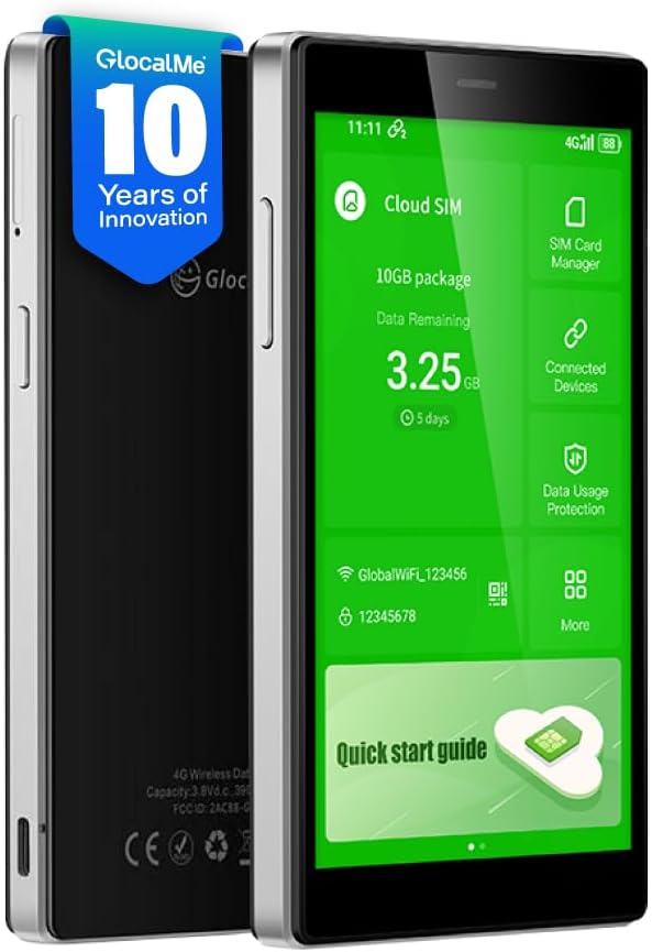
Glocalme Wi-Fi hotspot
Handy outside EU; keeps uploads working.
Buy on Amazon
This post contains affiliated links